BERT and the Attention Mechanism: How Transformers Actually Work

2018 was the year NLP changed. BERT landed in November and broke eleven benchmarks overnight. At the time I'd been using LSTMs for most sequence tasks, and the jump in performance felt almost unfair. It took me a while to properly understand why BERT worked so well — this is that explanation.

Why Earlier Models Weren't Enough

The RNN/LSTM era had one structural problem: information flowed in one direction. Even a bi-directional LSTM reads the sequence left-to-right and right-to-left separately, then concatenates the two hidden states. That concatenation doesn't let the model consider both sides simultaneously at every layer — it's an approximation.

Word embeddings (Word2Vec, GloVe) made things worse in a different way: the vector for "bank" was the same whether you were talking about a river bank or a financial institution. Context mattered, but the embedding didn't capture it.

ELMo introduced contextualised embeddings using a deep bi-directional LSTM, which helped. But it was still sequential and slow to train. The real shift came from abandoning recurrence entirely.

From Sequence to Attention

The Transformer (Vaswani et al., 2017) replaced recurrence with self-attention: for every token in a sequence, compute a weighted sum over all other tokens. The weights are learned — the model figures out which tokens should inform which.

$\text{Attention}(Q, K, V) = \text{softmax}\!\left(\frac{QK^T}{\sqrt{d_k}}\right) V$

Every token gets a Query ($Q$), Key ($K$), and Value ($V$) projection. The dot product of a token's Query against every other token's Key produces raw attention scores. Scaled by $\sqrt{d_k}$ and softmaxed, those become attention weights. The output is a weighted sum of all Value vectors.

This is computed in parallel for all tokens at once — no sequential bottleneck, and no information decay over distance.

BERT's Architecture

BERT uses only the encoder side of the original Transformer. No decoder, no autoregressive generation — just a stack of bidirectional encoder blocks.

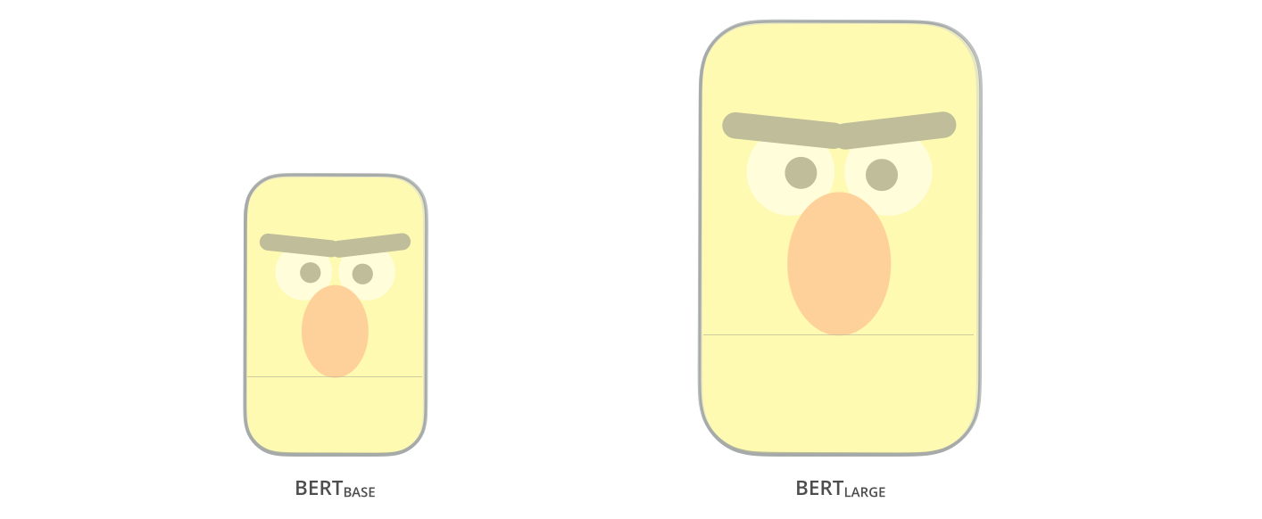
Two sizes were released:

Model	Encoder layers	Hidden size	Attention heads	Parameters
BERT Base	12	768	12	110M
BERT Large	24	1024	16	340M

Each layer is a standard Transformer encoder block: multi-head self-attention → layer norm → position-wise feed-forward → layer norm.

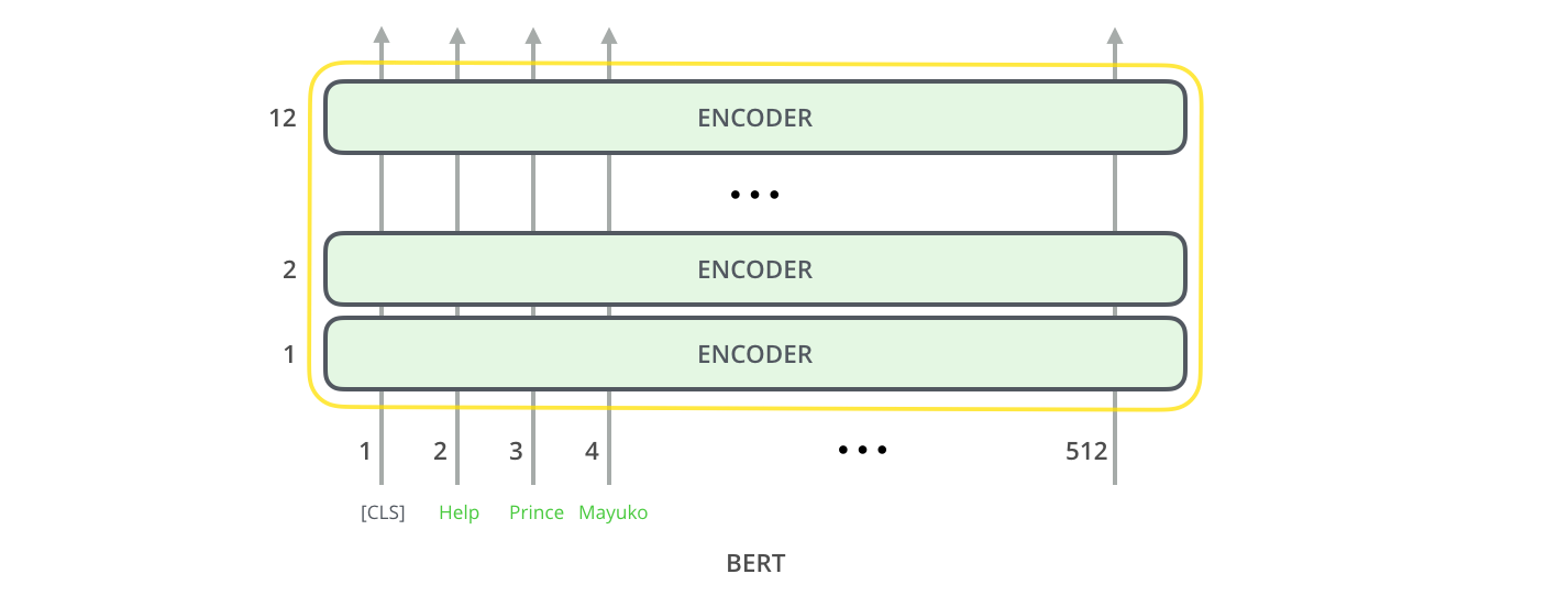
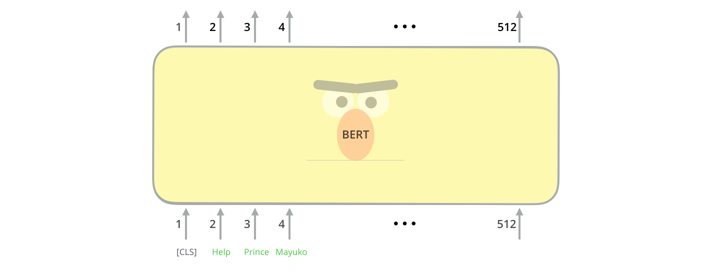
The input side has one important addition: a special [CLS] token is always prepended. Its output vector, after 12 (or 24) layers of attention, aggregates information from the entire sequence — this is what gets used for classification tasks.

The Pre-Training Trick: Masked Language Modelling

Here's the key insight. A language model that predicts the next word is inherently left-to-right — you can't look ahead. That makes it unidirectional. But BERT needs to be bidirectional from the start.

The solution: randomly mask 15% of input tokens, then train the model to predict the masked tokens from surrounding context in both directions.

In practice the 15% isn't always a [MASK] token — that would create a distribution shift between pre-training and fine-tuning (real text never has [MASK]). Of the 15% selected:

• 80% are replaced with [MASK]
• 10% are replaced with a random token
• 10% are left unchanged (but the model still has to predict the correct token)

This forces the model to develop robust representations rather than relying on the presence of a mask marker.

The Second Pre-Training Task: Next Sentence Prediction

BERT is also trained to understand relationships between sentences. Given two sentences A and B, the model predicts whether B actually follows A in the original text or is a random sentence.

50% of training pairs are genuine consecutive sentences; 50% are random. The [CLS] token's output vector is trained to encode this relationship. This is why [CLS] representations are so useful for downstream sentence-level tasks.

Transfer Learning: Pre-train Once, Fine-Tune Everywhere

The two-stage approach is what makes BERT powerful in practice:

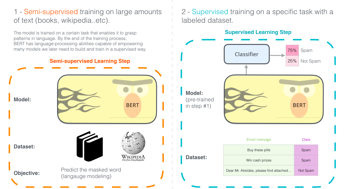
1. Pre-train on 3.3 billion words of BooksCorpus + English Wikipedia — no labels needed. This gives you a model that deeply understands language structure.
2. Fine-tune on your labelled task data — classification, NER, question answering — for a few epochs. The pre-trained weights are a warm start; you only need a small labelled dataset.

This is the ImageNet moment for NLP. Before BERT, every NLP project trained from scratch. After BERT, you download weights and fine-tune.

What BERT Can Do

After fine-tuning, BERT handles a remarkably wide range of tasks with the same underlying architecture:

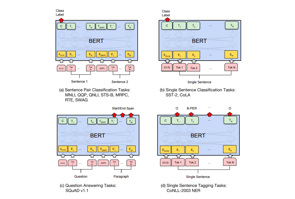
• Single sentence classification (sentiment, spam detection): add a linear classifier on the [CLS] output
• Sentence pair tasks (natural language inference, paraphrase detection): feed both sentences separated by [SEP], classify from [CLS]
• Token-level classification (named entity recognition): attach a classifier to every token's output vector
• Span extraction (question answering): predict start and end positions of the answer span

In every case the change to the BERT architecture is minimal — just a task-specific head on top.

Why This Works: A Practical Intuition

Multi-head attention is running 12 (or 16) attention patterns in parallel per layer. Empirical work on BERT's attention heads found that different heads specialise: some track subject-verb agreement, some track coreference, some track positional dependencies. No single head needs to capture everything.

After 12 layers, the contextualised representation of each token has been refined by attending to every other token 12 times, from multiple perspectives. The final representation of "bank" in "the river bank" and "the bank account" will be measurably different — the model has learned to disambiguate from context.

Getting Started with the Code

The full Python demo (in projects/bert-attention-mechanism/) loads BERT-base and visualises the attention weights for a sample sentence:

from transformers import BertTokenizer, BertModel
import torch

tokenizer = BertTokenizer.from_pretrained('bert-base-uncased')
model = BertModel.from_pretrained('bert-base-uncased', output_attentions=True)

sentence = "The bank deposited the money near the river bank."
inputs = tokenizer(sentence, return_tensors='pt')

with torch.no_grad():
    outputs = model(**inputs)

# outputs.attentions: tuple of 12 tensors, one per layer
# each tensor: (batch=1, heads=12, seq_len, seq_len)
attentions = outputs.attentions
print(f"Layers: {len(attentions)}, Shape per layer: {attentions[0].shape}")

Running that you get 12 attention matrices, one per layer, each showing which tokens each head attended to. Plotting layer 5, head 3 on the disambiguation sentence typically shows the two "bank" tokens attending to different contexts — a clean visual of what bidirectional attention actually learns.

What Came Next

BERT opened the floodgates. RoBERTa (2019) showed that training longer with more data and no NSP outperformed BERT. DistilBERT distilled it to 66M parameters with 95% of performance. ALBERT tied layer weights to cut parameters further. And GPT-2/GPT-3 showed that decoder-only models with enough scale could match BERT on many benchmarks too.

But the core idea — pre-train a deep bidirectional transformer on masked language modelling, then fine-tune — is still powering production NLP systems five years later. Understanding it is table stakes for any engineer working with language models.